The ETF Portfolio Strategist: 4 Nov 2021

Total Return Expectations

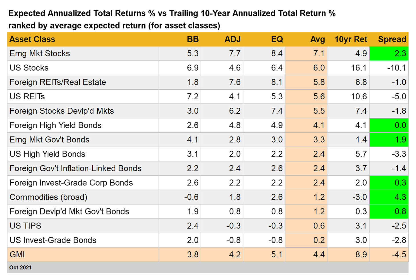
Total return expectations for the Global Market Index (GMI) continue to hold at 4%-plus, or roughly half the level of the index’s 10-year performance.

Today’s update of new total return forecasts for GMI through October show the benchmark’s ex ante performance ticked up to a 4.4% total return for the long term, slightly above the 4.3% estimate in last month’s outlook.

The main event for this data remains the wide gap between expectations and realized performance over the past decade. GMI — an unmanaged, market-value-weighted portfolio that holds all the major asset classes except cash — earned a strong 8.9% (annualized) over the trailing 10-year period through October 2021. Today’s estimate of the index’s long-term performance, by contrast, is about half that gain. For details on GMI’s design, see this summary.

Note, too, that several asset classes are currently posting expected returns above the 10-year trailing return (indicated by the green highlights in the far-right column. These positive spreads imply that the relevant markets are ripe for generating relatively higher returns in the years ahead.

Keep in mind, however, that the forecast for GMI is more reliable vs. the individual asset-class estimates. As with any forecast, it’s safe to assume that some projections will be too high, and some too low. Aggregating the forecasts via GMI provides a methodology to boost the probability — slightly — that the forecast is relatively accurate. On that basis, the highest confidence forecast in the table above is GMI’s outlook for substantially lower returns overall relative to the past decade.

Here are brief definitions for each column of data in the table above:

BB: The Building Block model uses historical returns as a proxy for estimating the future. The sample period used starts in January 1998 (the earliest available date for all the asset classes listed above). The procedure is to calculate the risk premium for each asset class, compute the annualized return and then add an expected risk-free rate to generate a total return forecast. For the expected risk-free rate, we’re using the latest yield on the 10-year Treasury Inflation Protected Security (TIPS). This yield is considered a market estimate of a risk-free, real (inflation-adjusted) return for a “safe” asset — this “risk-free” rate is also used for all the models outlined below. Note that the BB model used here is (loosely) based on a methodology originally outlined by Ibbotson Associates.

EQ: The Equilibrium model reverse engineers expected return by way of risk. Rather than trying to predict return directly, this model relies on the somewhat more reliable framework of using risk metrics to estimate future performance. The process is relatively robust in the sense that forecasting risk is slightly easier than projecting return. The three inputs:

1. An estimate of the overall portfolio’s expected market price of risk, defined as the Sharpe ratio, which is the ratio of risk premia to volatility (standard deviation). Note: the “portfolio” here and throughout is defined as GMI

2. The expected volatility (standard deviation) of each asset (GMI’s market components)

3. The expected correlation for each asset relative to the portfolio (GMI)

This model for estimating equilibrium returns was initially outlined in a 1974 paper by Professor Bill Sharpe. For a summary, see Gary Brinson’s explanation in Chapter 3 of The Portable MBA in Investment. I also review the model in my book Dynamic Asset Allocation. Note that this methodology initially estimate risk premium and then adds an expected risk-free rate to arrive at total return forecasts. The expected risk-free rate is outlined in BB above.

ADJ: This methodology is identical to the Equilibrium model (EQ) outlined above with one exception: the forecasts are adjusted based on short-term momentum and longer-term mean reversion factors. Momentum is defined as the current price relative to the trailing 12-month moving average. The mean reversion factor is estimated as the current price relative to the trailing 60-month (5-year) moving average. The equilibrium forecasts are adjusted based on current prices relative to the 12-month and 60-month moving averages. If current prices are above (below) the moving averages, the unadjusted risk premia estimates are decreased (increased). The formula for adjustment is simply taking the inverse of the average of the current price to the two moving averages. For example: if an asset class’s current price is 10% above its 12-month moving average and 20% over its 60-month moving average, the unadjusted forecast is reduced by 15% (the average of 10% and 20%). The logic here is that when prices are relatively high vs. recent history, the equilibrium forecasts are reduced. On the flip side, when prices are relatively low vs. recent history, the equilibrium forecasts are increased.

Avg: This column is a simple average of the three forecasts for each row (asset class)

10yr Ret: For perspective on actual returns, this column shows the trailing 10-year annualized total return for the asset classes through the current target month (July 2021 in this case).

Spread: Trailing 10-year return less model-average forecast. ■